Sample Exercises

By M. Vreeswijk, University of Amsterdam (8 points)

Maxwell's laws are as follows:

• electrostatics:
• \(\oint\limits_{circle}\overrightarrow{E}\cdot d\overrightarrow{l} = 0\)
• \(\Phi_{E}\equiv \oint\limits_{surface}\overrightarrow{E}\cdot d\overrightarrow{o} = \frac{Q^{enclosed}}{\epsilon_{0}}\)
• magnetostatics:
• \(\oint\limits_{circle}\overrightarrow{B}\cdot d\overrightarrow{l} = \mu_{0}I^{enclosed}\)
• \(\Phi_{B}\equiv \oint\limits_{surface}\overrightarrow{B}\cdot d\overrightarrow{o} = 0\)

Figure 1.1: The amount of charge in the origin

In the origin of our coordinate system, we find an amount of electrical charge: $Q(t)=Q_{0}e^{\frac{-t}{\tau}}$

where $t$ is the time, $\tau$ is a constant and $Q_0$ is the charge at time $t=0$.

1 Calculate, using Gauss' law, the electrical field that is induced by the charge in the origin. Indicate with a drawing which 'Gaussian surface' you've used.

The electrical charge in the origin can't just disappear. We presume that the charge moves away (flows) in a radial direction.

2. Give an expression for the electric current $I(t)$ and the density current $\overrightarrow{J}$. (Be aware that the density current is a vector and therefore, it has a direction.)

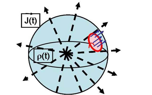
3. Argue, by use of a symmetry argument, there can't be a magnetic field parallel to the surface of the imaginary ball in Figure 1.1.

4. Argue, if necessary with the Ampère's circuital law, that there's a magnetic field parallel to the surface of the ball. You could be inspired by the Ampère loop which is included in Figure 1.1.

The answers given in 3. and 4. are, as you might have noticed, contradictionary. Luckily, we all know that Maxwell solved this contradiction in a brilliant fashion, by adding a term to Ampère's circuital law.

5. Give Ampère's circuital law as an integral, with Maxwell's addition. Show that, with this extra term, the magnetic field at 4. will disappear as well. (Hint: use answers found at 1. and 2.)

By Hans Jordens, University of Groningen (9 points)

In the northern part of the Dutch province Groningen, extensive research is done to noise caused by F16's. The terrain where the investigation takes place, is open. At a certain moment, the F16 is spotted, flying at constant height towards the observers. Directly after seeing the F16, a recording device is turned which measures the spectrum of sound during a period of time. The frequency of the loudest tone is shown in the graph, as a function of time. The minimum height at which an F16 is allowed to fly, is known to be 1000 ft. We neglect the absorption of sound.

The following is known:
The speed of sound through air is $343 \text{ ms}^{-1}$
$1 \text{ ft} = 0.3048 \text{ m}$

Determine, using the data in Figure 2.1
1. The speed of the F16,
2. The frequency of the loudest tone in the recorded spectrum,
3. Whether or not the F16 flies above 1000 ft,
4. The horizontal distance at which the F16 was first noticed.
Please clarify how you calculate your results.

Figure 2.1: The recorded frequency (Hz) as a function of time (s)

By R.A. Duine, Utrecht University (11 points)

Consider an electrical conductor, which has a temperature difference $\Delta T$ and a voltage difference $\Delta V$.

1. Start with a temperature difference equal to zero ($\Delta T = 0$) and presume that the electrical current $I$ is determined by Ohm's Law: $I = \Delta V R^{-1}$, with $R$ the resistance of the conductor. Use the first law of Thermodynamics, $dU = dQ + \mu dN = T dS + \mu dN$ (where $dU$ : change of energy, $dQ$ the heat, $\mu$ : the chemical potential, $dN$ : the change of particles $T$ the temperature and $dS$ the change of entropy), to show that the total heat, produced by the electric current per time unit, is given by: \begin{equation} \frac{dQ}{dt}=\frac{\Delta V^{2}}{R} \end{equation}

2. Let us now discuss the situation $\Delta V = 0$, $\Delta T = 0$. Now we find an electric current $I$, as well as an heat wave $I_{Q}$ through the conductor. Presume that: \begin{equation} I=\frac{\Delta V}{R}-\frac{S \Delta T}{R} \end{equation} and \begin{equation} I_{Q}=\frac{P \Delta V}{R}-\kappa^{'}\Delta T \end{equation} Here $S$ is the so called Seebeck coefficient and $P$ the Peltier coefficient. Furthermore $\kappa^{'}$ is the thermal conductivity at $\Delta V=0$. Use the First Law to show that: \begin{equation} \frac{dQ}{dt}=\frac{\kappa^{'} \Delta T^{2}}{T}+\frac{\Delta V^{2}}{R}-\frac{P \Delta V \Delta T}{RT}-\frac{S \Delta V \Delta T}{R} \end{equation}

3. Use the Second Law of Thermodynamics to show that the transport coefficients must satisfy: $\kappa^{'}R \geq PS$

By J. van Dongen & D. Dieks, Utrecht University (10 points)

In 1908 Paul Ehrenfest proposed a paradoxal case to physicists who were working on the, then new, special theory of relativity. The problem gave birth to lots of discussion and inspired Albert Einstein to further develop his theory.

Ehrenfest had the following in mind:

A rigid body in the shape of a cilinder, height $H$, radius $R$ and circumference $O$, $(O = 2\pi R)$, is initially at rest and is then put into a circular movement around it's axis. From a certain point the cilinder rotates with a constant angular speed. An observer who moves along with the cilinder will measure a radius $R^{'}$ and a perimeter $O^{'}$.

1. What do you expect, according to the theory of special relativity, to be the ratio between $R^{'}$ and $O^{'}$.

2. What do you think is problematic in this particular case?

3. Try to give your own analysis on what's happening to the cylinder.

By Han Velthuis, TNO Fluid Dynamics (8 points)

Consider a long, round pipe with water flowing through. The inner radius of the pipe is $R=0.025 \text{ m}$. The length of the pipe is $L = 1 \text{ km}$. We presume that the flow through the pipe is stationary, i.e. that the velocity profile of the water in the pipe isn't changing as a function of time nor as a function of the coordinate in the flow direction. The velocity profile $u(r)$ is purely a function of the radius $r$, where the radius is measured from the axis of the pipe. The variable $u$ depicts the velocity of water. The pressure drop over the pipe length $L$ is represented by variable $\Delta p$.

• Beneath a critical value the flow will be laminar. Solving the theoretical equations of flow (Navier-Stokes, 1822) will give a parabole as velocity profile. The speed of water will be zero near the side ($r=R$), and maximal at the axis ($r=0$).
• Above a critical value the flow will be turbulent. The turbulent velocity profile is often described with the so called 'power-law', where the velocity profile is proportional with $(Y/R)^c$. Here $y$ is the distance to the side and $c$ is a constant (say $c = \frac{1}{7}$).
• The critical value is given by the so called Reynolds number $Re = \frac{\rho~u_{ave}D}{\mu}$, named after the famous British scientist Osborne Reynolds (1842-1912). Here $\rho$ is the density of water, $D$ is the inner diameter of the pipe and $\mu$ is the dynamic viscosity of water.

Questions:
1. Derive an expression for the loss of pressure $\Delta p$ along the pipe as a function of the shear stress $\tau$ at the side of the wall.
2-a. Construct a graph of this pressure drop along the pipe as a function of the average velocity of water, $u_{ave}$, with the reach of velocity $u_{ave} \in [0,0.1] \text{ ms}^{-1}$. Use the CRC handbook to find the correct properties of water.
(Hint: In order to determine the shear stress, one has to determine the shape of the velocity profile as a function of the radius $r$).
2-b. Why is it impossible to construct the entire graph?
3-a. An emperical formula of turbulent pressure drop along the pipe $\Delta p$ is given by: \begin{equation} \Delta p=\frac{0.3164}{(Re)^{0.25}} \frac{L}{2R} \frac{1}{2}\rho u_{ave}^2 \end{equation} What's the graph now?
3-b. What's striking about this graph?

By G.A. Blab, Utrecht University (10 points)

Figure 6.1: Simplified Jabłónski diagram of a fluorescent molecule. A photon $h\nu_1$ can excite the molecule from its ground state $\left|S_0\right>$ to an excited state $\left|S_1\right>$. From there, the molecule can emit a photon with lower energy $h\nu_2$ and go back to the ground state, or makes an transition through a triplet (dark) state $\left|T\right>$ back to the ground state, or bleach to become a photo product $\left|B\right>$. When asked for a numerical answer, use the following rate constants: radiative $k_\mathrm{F}= 3 \times 10^{8} \text{ s}^{-1}$; non-radiative $k_\mathrm{V} = 1 \times 10^{12} \text{ s}^{-1}$, $k_\mathrm{ISC}= 1 \times 10^{7} \text{ s}^{-1}$, $k_\mathrm{T}= 2 \times 10^{5} \text{ s}^{-1}$, $k_\mathrm{bl}= 1 \times 10^{4} \text{ s}^{-1}$.

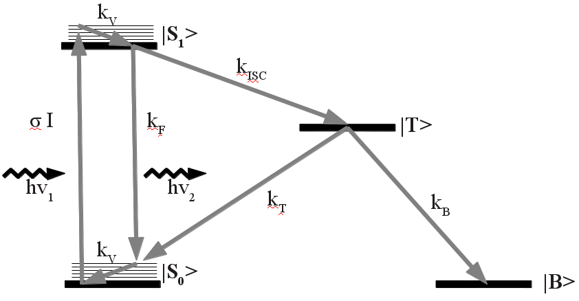
1. Find an analytical expression for the measured fluorescence life time $\tau_\mathrm{F}$, that is the life time of the excited state $\left|S_1\right>$ after absorption of a photon $h\nu_1$. From the general expression, make the assumption $k_\mathrm{V} \gg k_\mathrm{F}, k_\mathrm{ISC}$. How does this effective fluorescence life time $\tau_\mathrm{F}$ differ from $(k_\mathrm{F})^{-1}$?

2. Ignoring for the moment the irreversible bleaching, what is the expected time constant for one excitation emission cycle $\tau_\mathrm{cycle}$? What does this mean for the number of photons a molecule can emit per unit time? You may use the approximation $k_\mathrm{ISC}\gg k_\mathrm{T}$ in your calculations.

3. Find the excitation intensity (expressed in $\text{ W cm}^{-2}$) needed for a photon emission(!) rate of $5 \times 10^{4} \text{ s}^{-1}$ from a single molecule. To find the absorption cross section $\sigma$, you may assume that the condition are such that the Beer-Lambert law is valid and that the molar extinction coefficient of the fluorophore is $\epsilon= 80000 \text{ M}^{-1} \text{cm}^{-1}$ at the excitation wavelength $\lambda_\mathrm{exc}= 488 \text{ nm}$.